Upper Limits

Understanding RooStats

I will use RooStats RooStats in order to set an upper limit on the :

python -c 'import sphinx'

If that fails grab the latest version of and install it with:

> sudo easy_install -U Sphinx

Now you are ready to build a template for your docs, using sphinx-quickstart:

> sphinx-quickstart

accepting most of the defaults. I choose “sampledoc” as the name of my project. cd into your new directory and check the contents:

home:~/tmp/sampledoc> ls
Makefile      _static         conf.py
_build                _templates      index.rst

The index.rst is the master ReST for your project, but before adding anything, let’s see if we can build some html:

make html

If you now point your browser to _build/html/index.html, you should see a basic sphinx site.

Bayesian Approach

Now we will start to customize out docs. Grab a couple of files from the web site or svn.

The last step is to modify index.rst to include the getting_started.rst file (be careful with the indentation, the “g” in “getting_started” should line up with the ‘:’ in :maxdepth:

Contents:

.. toctree::
   :maxdepth: 2

   getting_started.rst

and then rebuild the docs:

cd sampledoc
make html

Frequentist Approach

#
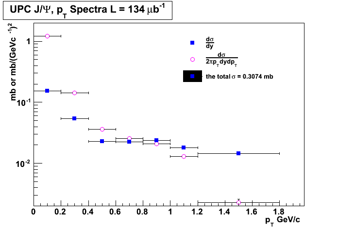
#Guillermo Breto Rangel UPC xsection vs root(s)
#
import math
from ROOT import TCanvas, TGraph, TGraphErrors, TF1, TLegend
from ROOT import gROOT
from math import pow
from array import array

gROOT.Reset()

c1 = TCanvas( 'c1', 'A parameter as funtion of \sqrt{s}', 400, 400, 700, 500 )

#c1.SetFillColor( 42 )
#c1.SetGrid()

#n = 3
lumi = 134000
p_T = array( 'd',[0.1, 0.3, 0.5, 0.7, 0.9, 1.1, 1.5] )
yields_dpT = array( 'd',[3062,2989,6050, 2426, 1687] )
dsigma_dy = array( 'd',[20539./lumi,7251./lumi,3062./lumi,2989./lumi,3191./lumi, 2426./lumi, 1734./lumi] )
err_x = array( 'd',[0.1, 0.1, 0.1, 0.1, 0.1, 0.1, 0.3])
err_y = array('d',[167./lumi, 70./lumi, 56./lumi, 56./lumi, 59./lumi, 50./lumi, 42./lumi])

def cross_section(eff, lumi, weighted_jpsi_yield):
    xsection = weighted_jpsi_yield/(eff*lumi)
    return xsection

lumi = 134/math.pow(10,-3)
eff_list = [1, 0.98, 0.95, 0.90, 0.85, 0.80]

weighted_jpsi_yield = round(sum(dsigma_dy),4)*lumi

for i in range(len(eff_list)):
    eff = eff_list[i]
    print "The value of the cross section for ", eff*100,"% efficiency is ", round(cross_section(eff,lumi,weighted_jpsi_yield),3), "mb"



print "the total cross ssection is", round(sum(dsigma_dy),4)
print dsigma_dy
n = len(p_T)
gr_dsigma_pT = TGraphErrors(7)

for i in range(7):
    gr_dsigma_pT.SetPoint(i,p_T[i],dsigma_dy[i]/(2.0*math.pi*0.2*p_T[i]))
    print p_T[i]
    print dsigma_dy[i]/(0.2*p_T[i])
    gr_dsigma_pT.SetPointError(i, 0.1, err_y[i])
    if (i == n - 1):
        gr_dsigma_pT.SetPoint(i,p_T[i],dsigma_dy[i]/(2.0*math.pi*0.6*p_T[i]))
        gr_dsigma_pT.SetPointError(i, 0.3, err_y[i])

gr = TGraphErrors(7)

for i in range(7):
    gr.SetPoint(i,p_T[i],dsigma_dy[i])
    gr.SetPointError(i, 0.1, err_y[i])
    if (i == n - 1):
        gr.SetPoint(i,p_T[i],dsigma_dy[i]/(0.6*p_T[i]))
        gr.SetPointError(i, 0.3, err_y[i])


#gr = TGraphErrors( 7, p_T, dsigma_dy, err_x, err_y )
#gr.SetLineColor( 2 )
gr.SetLineWidth( 1 )
gr_dsigma_pT.SetLineWidth( 1 )
gr_dsigma_pT.SetMarkerColor(6)
gr.SetMarkerColor( 4 )
gr.SetMarkerStyle( 21 )
gr_dsigma_pT.SetMarkerStyle( 24 )

gr.SetTitle( 'p_{T} Spectra' )
gr_dsigma_pT.SetTitle( 'UPC J/#Psi, p_{T} Spectra L = 134 #mub^{-1}' )

gr.GetXaxis().SetTitle( 'p_{T} GeV/c' )
gr_dsigma_pT.GetXaxis().SetTitle( 'p_{T} GeV/c ' )

gr.GetXaxis().SetRangeUser(0, 2)
#c1.SetLogx()
gr.GetYaxis().SetTitle( '#frac{d#sigma}{dy} (#mub)' )
gr_dsigma_pT.GetYaxis().SetTitle( 'mb or mb/(GeVc^{-1})^{2}' )
gr.GetYaxis().SetTitleOffset(1.2)
gr.GetYaxis().SetRangeUser(0, 10)
gr_dsigma_pT.GetYaxis().SetRangeUser(-10, 2)

gr_dsigma_pT.Draw('AP')
gr.Draw("psame")
#gr_dsigma_pT.Draw('same')
c1.SetLogy()

leg = TLegend(0.53,0.63,0.85,0.85)
leg.SetBorderSize(0)
leg.SetFillColor(0)
leg.SetTextSize(0.03)
leg.AddEntry(gr,"#frac{d#sigma}{dy}","P")
leg.AddEntry(gr_dsigma_pT,"#frac{d#sigma}{2#pip_{T}dydp_{T}}","P")
leg.AddEntry(gr, "the total #sigma = "+ str(round(sum(dsigma_dy),4))+" mb")
leg.Draw('same')

# TCanvas.Update() draws the frame, after which one can change it
c1.Update()
#c1.GetFrame().SetFillColor(0)
#c1.GetFrame().SetBorderSize( 12 )
#c1.Modified()
#c1.Update()
c1.Print('UPC_pt_graphlog.png')
c1.Print('UPC_pt_graphlog.pdf')

(Source code)

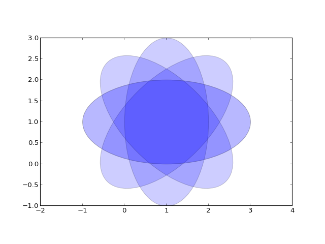
Inserting automatically-generated plots is easy. Simply put the script to generate the plot in the pyplots directory, and refer to it using the plot directive. First make a pyplots directory at the top level of your project (next to :conf.py) and copy the ellipses.py` file into it:

home:~/tmp/sampledoc> mkdir pyplots
home:~/tmp/sampledoc> cp ../sampledoc_tut/pyplots/ellipses.py pyplots/

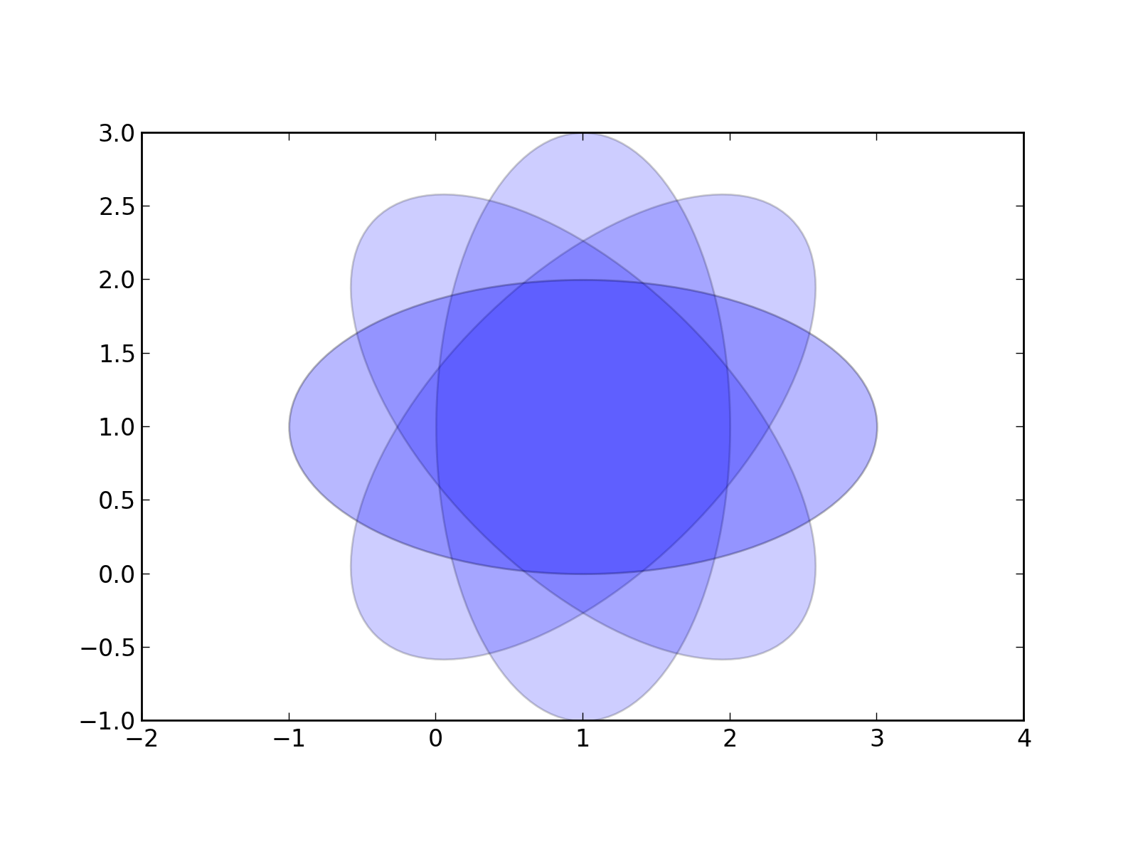
You can refer to this file in your sphinx documentation; by default it will just inline the plot with links to the source and PF and high resolution PNGS. To also include the source code for the plot in the document, pass the include-source parameter:

.. plot:: pyplots/ellipses.py
   :include-source:

In the HTML version of the document, the plot includes links to the original source code, a high-resolution PNG and a PDF. In the PDF version of the document, the plot is included as a scalable PDF.

from pylab import *
from matplotlib.patches import Ellipse

delta = 45.0 # degrees

angles = arange(0, 360+delta, delta)
ells = [Ellipse((1, 1), 4, 2, a) for a in angles]

a = subplot(111, aspect='equal')

for e in ells:
    e.set_clip_box(a.bbox)
    e.set_alpha(0.1)
    a.add_artist(e)

xlim(-2, 4)
ylim(-1, 3)

show()

(Source code, png, hires.png, pdf)

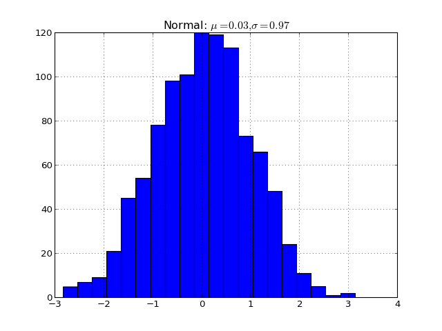
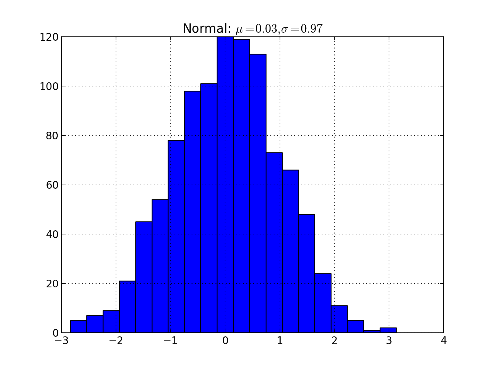
You can also inline code for plots directly, and the code will be executed at documentation build time and the figure inserted into your docs; the following code:

.. plot::

import matplotlib.pyplot as plt import numpy as np x = np.random.randn(1000) plt.hist( x, 20) plt.grid() plt.title(r’Normal: $mu=%.2f, sigma=%.2f$’%(x.mean(), x.std())) plt.show()

produces this output:

(Source code, png, hires.png, pdf)

See the matplotlib pyplot tutorial and the gallery for lots of examples of matplotlib plots.

When you reload the page by refreshing your browser pointing to _build/html/index.html, you should see a link to the “Getting Started” docs, and in there this page with the screenshot. Voila!

Note we used the image directive to include to the screenshot above with:

.. image:: _static/basic_screenshot.png

Next we’ll customize the look and feel of our site to give it a logo, some custom css, and update the navigation panels to look more like the sphinx site itself – see Customizing the look and feel of the site.