Compton Scattering

 

by Roppon Picha (69769577)

Lab Partner: Jiro Oi

Instructor: Professor Rutledge

Physics 121

Winter 2000

 

    Compton scattering is the scattering of a photon by a massive particle such as an electron. This experiment illustrates the photon (particle) nature of light, first performed in 1923 by Sir Arthur H. Compton. The gamma ray is scattered of an electron in a material. Observing that the scattered light had a wavelength different than the incident light, Compton realized that the wave model of light cannot explain the event. In the wave picture, the frequency does not change upon impact or transition between media. The only explanation for the change in photon frequency is that light are particles. Compton explained and modeled the data by assuming a particle nature for light and applying conservation of energy and conservation of momentum to the collision between the photon and the electron. The scattered photon has lower energy and therefore a longer wavelength according to the Planck relationship. According to Compton’s speculation, light is a group of photons, with each photon containing energy . Compton analyzed and found momentum of light to be . From , we calculated the energy of the scattered photon. The Compton experiment gave clear and independent evidence of particle-like behavior. In 1927 Compton was awarded the Nobel Prize for the discovery.

 

We use cesium (atom. no. 55, isotope mass 137) as the gamma source. The incident photon collides with electron in aluminum (Fig. 1).

 

By the conservation of energy,

 

    -----     (Eq. 1)

 

Where h = Planck’s constant = 6.626 x 10 -34 J s; v = frequency of incident photon; m = mass of electron = 9.31 x 10 -31 kg, c = speed of light = 3 x 10 8 m/s; = frequency of deflected photon; p = momentum of recoiled electron.

 

From the conservation of momentum,

 

    -----     (Eq. 2)

    -----     (Eq. 3)

 

Where = angle of scatted photon; = angle of recoiled electron.

 

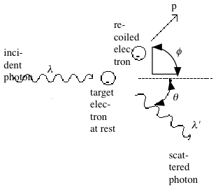
Fig. 1: Compton scattering of a photon by a stationary electron. (Collision between the photon and the electron causes the deflected photon to have lowered energy.)  

 

From equations 1, 2, and 3, we obtain

 

    -----     (Eq. 4)

 

Where and are wavelengths of incident and scattered photon, respectively.

 

This gives us the energy of the scattered photon ,

 

    -----     (Eq. 5)

 

Where E = peak energy or incident energy, which for Cs-137 is 662 keV.

 

From this equation we obtain predicted energy at different angles (Table 1).

 

 angle (degree)      E predicted (keV)

    0            662

    20            614.1478463

    30            564.3188548

    40            508.340416

    50            452.9471919

    60            402.1754562

    70            357.7986691

    80            320.1460074

    90            288.7986331

    100            263.0393223

    110            242.0979163

    120            225.2668273

    130            211.9450146

    140            201.6468414

    150            193.9959427

 

Table 1: Predicted energy at different scattering angles, according to Compton formula (Eq. 5)

 

Plot these results we get the graph in (Fig. 2).

 

 

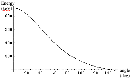
Fig. 2: Predicted energy vs angle

 

 

    At peak energy ( ), 662 keV corresponded to channel number 1792. We measured energy of another radioactive substance which gives out photon of energy 511 keV, we found the energy to be at channel 1362. Since we only have two materials to calibrate, and the error of the second material (from the predicted channel 1383.25) is only 1.536%, we assume the relationship of channel-energy to be linear, passing through the origin (Fig. 3).

 

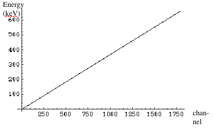
Fig. 3: Energy vs channel

 

 

 

 

 

 

 

 

 

We measured energy at different angles and obtained the results (Table 2).

 

  angle (degree)    channel   E experiment (keV)  meas error    % deviation

    0        1792    

    20        1642        606.5870536          8.13        +1.231

    30        1520        561.5178571          7.11        +0.496

    40        1357        501.3024554          7.39        +1.385

    50        1227        453.2779018          2.96        -0.073

    60        1089        402.2979911          1.85        -0.030

    70        960        354.6428571          1.85        +0.882

    80        869        321.0256696          4.06        -0.275

    90        785        289.9944196          4.8            -0.414

    100        714        263.765625          1.48        -0.276

    110        663        244.9252232          3.32        -1.168

    120        616        227.5625          6.28        -1.019

    130        581        214.6328125          4.06        -1.268

 

Table 2: Experimental results of energy at different angles. (Calculated from corresponding channels, assuming linear relationship between channel-energy (Fig. 3).)

 

Plot the results and we obtain the graph in (Fig. 4).

 

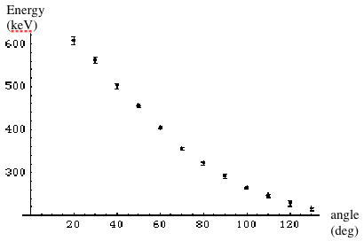
Fig. 4: Experimental energy vs angle

 

 

 

 

 

 

 

 

 

 

 

 

 

 

The results agree well with the theory (Eq. 5). See (Fig. 5).

 

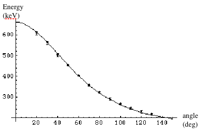
Fig. 5: Experimental energy and theoretical energy

 

Also, from (Eq. 5) we have

 

    -----     (Eq. 6)

 

See (Fig. 6). The linear fit equation of the plot is

 

y = 0.00153843+0.0019055x     -----     (Eq. 7)

 

Where y = 1/E; x = (1-cos ).

 

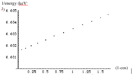
Fig. 6: 1/E vs (1-cos ), expected to be linear according to (Eq. 6). The slope of the plot is .

Slope 0.0019055 is in good agreement with the actual value of = 0019536 keV -1 .

 

    Lastly, we evaluate the differential cross section. Using efficiency data of NaI crystal 1-inch diameter x 1-inch thick (actual diameter = 1.5 inches), we calculate the corrected yield from the experiment (Table 3).

 

angle (degree)    yield (counts/sec)    efficiency    corrected yield

    0            

   20            6.147704591            0.47            13.080222534

   30            4.644455495            0.49            9.478480602

   40            4.153037962            0.52            7.9866114654

   50            3.309937789            0.55            6.0180687073

   60            3.029146592            0.6            5.0485776533

   70            2.356760886            0.65            3.6257859785

   80            2.157219063            0.69            3.1264044391

   90            2.018568012            0.72            2.8035666833

  100            2.210626186            0.75            2.9475015813

  110            2.156776878            0.78            2.7650985615

  120            2.329278408            0.81            2.8756523556

  130            2.449510664            0.84            2.9160841238

 

Table 3: Count rates (yields) at different angles

 

This gives us the plot in (Fig. 7).

 

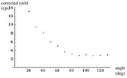
Fig. 7: Yield vs angle

 

Using the cross section equation

 

    -----     (Eq. 8)

 

Where yield = counts/second; = detector’s solid angle element = = 7.07 x 10 -3 sr.

N = the total number of electrons in the aluminum target.

 

    -----     (Eq. 9)

 

Where d = target’s diameter = 2.8 cm; h = target’s height = 9 1 cm; = aluminums density = 2.7 g/cm 3 ; = Avogadro’s number = 6*10 23 ; A = atomic weight of aluminum= 27; Z = atomic number of aluminum = 13.

 

Therefore N = 4.32 x 10 25 electrons.

 

is the flux density at the target = , where peak counts = maximum flux at zero degree = 4394.7 2.4 counts/cm 2 -s; = crystal detector efficiency at zero degree = 0.47; r = distance between source and detector = 2 r’; r’ = distance between source and target.

 

Thus = 3.74 x 10 4 photons/cm 2 -s.

 

From (Eq. 8) and corrected yield data, we obtain

 

    -----     (Eq. 10)

 

There are 2 models that predict the differential cross section of the Compton scattering. The first is the Thomson formula, solely dependent on the angle

 

    -----     (Eq. 11)

 

Where is the so-called “classical electron radius” = 2.82 x 10 -13 cm.

 

The other formula is called Klein-Nishina formula, which takes frequency into account

 

    -----     (Eq. 12)

 

Where = 1.293, for = 662 keV.

 

The scattering cross section as a function of angle according to Thomson model and Klein-Nishina model, along with our experimental results, is shown in (Fig. 8).

 

 

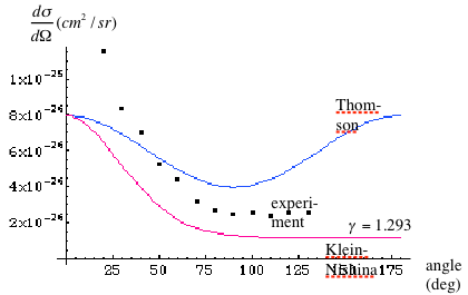
Fig. 8: The scattering cross section as a function of angle. Althought with offset, the experimental results seem to agree with Klein-Nishina, as expected.

 

The Klein-Nishina explains the cross section of high-energy photons better than Thomson, which ignores the frequency factor. The shape of experimental data plot looks like the Klein-Nishina, despite the offset. The offset may be due to large error from the estimates of the flux density and the total number of electrons.

 

______________________________