Monte Carlo sampling

Fundamental THEOREM for sampling.-
Consider the probability distribution $\frac{dP(x)}{dx}$, i.e.,
$dP(x)$ = probability for $x$ to be between $x$ and $x+dx$.
Assume also, for generality, that $x$ is limited to the interval ($x_{min}$, $x_{max}$).
Then, the THEOREM says that the cummulative normalized distribution is a uniform distribution:

$$\begin{eqnarray*} \frac{\int_{x_{min}}^x dP(t)} {\int_{x_{min}}^{x_{max}} dP(t)... ... r \ ,r uniform in (0,1) (1) \\ \end{eqnarray*}$$

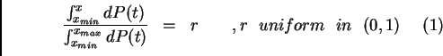
See Figure in Appendix of Green (reference at bottom), which illustrates the equipartition of areas implict in eq. (1)

We don't prove this result, which for some people can be considered "manifestly true."
We verify in eq. (1) that for $x=x_{min}, r=0$, and for $x=x_{max}, r=1$, that is, distribution (1) satisfy the limits corresponding to the variable $r$.

The THEOREM tell us that the desired value $x$ is obtained by solving ("inverting") eq. (1) for $x$.

A) We next discuss some cases of interest that can be solved analytically, i.e., $x$ can be expressed explicitily as a function of $r$.

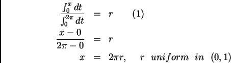
1) The distribution is uniform in the interval, for instance, the case of the azimuthal angle $0<\phi<2\pi$ in scattering.

$$\begin{eqnarray*} \frac{\int_{0}^x dt} {\int_{0}^{2\pi} dt} &=& r (... ...&=& r \\ x &=& 2\pi r, r uniform in (0,1) \end{eqnarray*}$$

2) Polar angle $\theta$ for Rutherford scattering for small angles.

$$\begin{eqnarray*} \frac{dP(\theta)} {d\theta} &=& K \frac{1}{\theta^4}, or,... ...ha+1})}]^\frac{1}{\alpha+1}, r uniform in \ (0,1) \end{eqnarray*}$$

Note that
a) The multiplicative factor in the distribution is not relevant for the sampling.
b) For the case $\alpha=0$, the distribution reduces to the uniforme distribution, as it should be.

3) Mean free path $\Lambda$ (or, also, radiactive or particle decay). These cases correspond to an exponential distribution $\frac{dP(x)}{dx} = K \exp{\frac{-x}{\Lambda}}$:

$$\begin{eqnarray*} \frac{\int_{x_{min}}^x K e^-(t/\Lambda) dt} {\int_{x_{min}}... ...ac{x_{min}}{\Lambda}})], r uniform in (0,1) \par\end{eqnarray*}$$

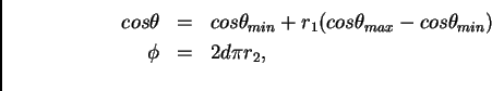
4) Isotropic angular distribution.- $\frac{d\sigma}{d\Omega}=const$, that is, we would like to send, on the average, the same number of particles into each solid angle .

$$\begin{eqnarray*} d\Omega = sin \theta d\theta d\phi = d(cos \theta) d\phi \end{eqnarray*}$$

We have expressed here the element of solid angle $d\Omega$ as the product of two independent variables, each one with a uniform distribution. For $0<\phi<2\pi$ and $\theta_{min}<\phi<\theta_{max}$, we get, from (1):

$$\begin{eqnarray*} cos\theta &=& cos \theta_{min} + r_1 (cos \theta_{max}-cos \theta_{min}) \\ \phi &=& 2 d\pi r_2, \\ \end{eqnarray*}$$

where $r_1$ y $r_2$ are two random numbers uniformly distributed in the unit interval (0,1).

B) If the distribution to be sampled does not have an inverse, that is, if $x$ can not be (easily) expressed as a function of $r$, it is always possible to use a method of trial and error that eventually gives us a value of $x$ with the distribution we are looking for. This computational method is known as the "acceptance/rejection method". See, for instance, the Appendix to Green or the Particle Data Book.

REFERENCES
Dan Green, "The Physics of Particle Detectors", Cambridge University Press, 2000. See Appendix K, "Monte Carlo models", p. 348.
Particle Data Group, "Review of Particle Physics", Phys. Rev. D, 66,01001-1 (2002). See "32. Monte Carlo Techniques"