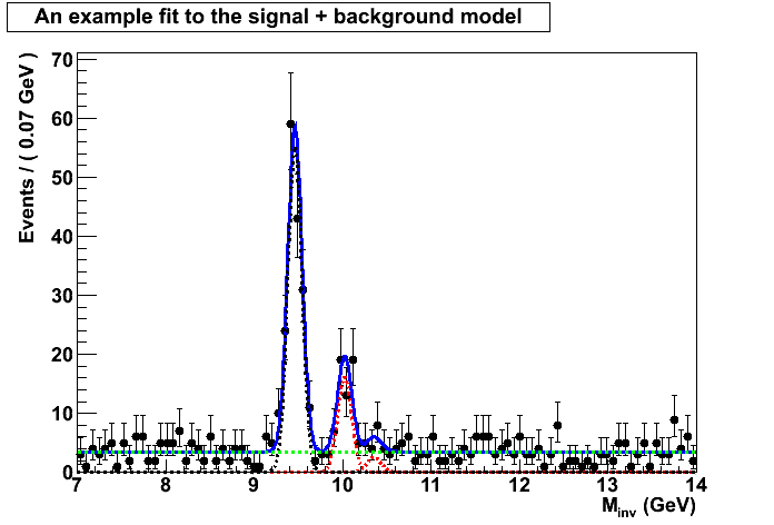
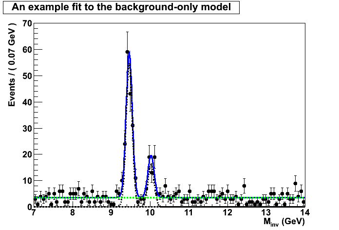
This is a project I performed trying to make some inferences on the
 state. For this example I chose a Chevychev
polynomial background and my three upsilon peaks. I tuned the
third peak to be almost not present and then measured the p-value
of the null hypothesis (the third peak is not there).
state. For this example I chose a Chevychev
polynomial background and my three upsilon peaks. I tuned the
third peak to be almost not present and then measured the p-value
of the null hypothesis (the third peak is not there).
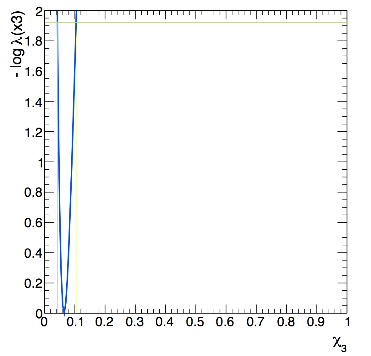
ProfileLikelihood Calculator (roostats)
nominal case / no systematics:
using the entire mass range 7-14
Floating Parameter FinalValue Error beta_nbkg 0.0000e 6.50e-01
f1S 3.0730e-01 f2S 6.0212e-02 glob_nbkg 0.0000e+00 mu 1.2701e+00 x3 1.5401e-02
Significance:
The p-value for the null is 0.205407
Corresponding to a signifcance of 0.822464
Note
As you can see the p-value is very large so the significance of the peak above the background is very small and we can’t reject the null hypothesis even though we know the signal 3S is present. No discovery!
No discovery but we can do better. We can set up an upper limit on the signal for the third peak. Now there are two ways to approach this problem. We can either applying a Bayesian approach or a frequentist approach.
For the purpose of this exercise I followed bothe approaches but you should be aware of their difference. The frequentist claim that there’s an unkown true parameter which we should be able to cover with the upper limit estimation. The Bayesian approach however assigns a probability the unknown parameter and, hence, applying Bayesian theorem assigns a prior probability to our parameter of interest in this case the yield of the third peak. To be precise, I will instead of setting a limit on the yield I will set a limit on the fraction of the third peak with respect to the first peak.
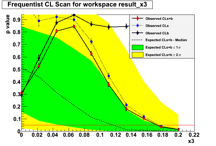
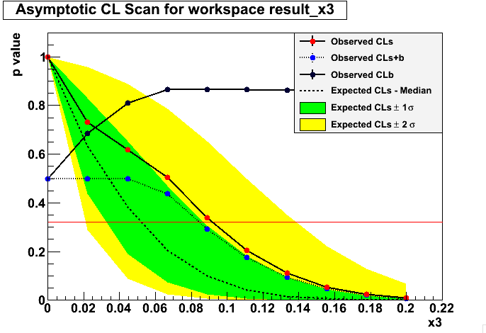
Frequentist approach:
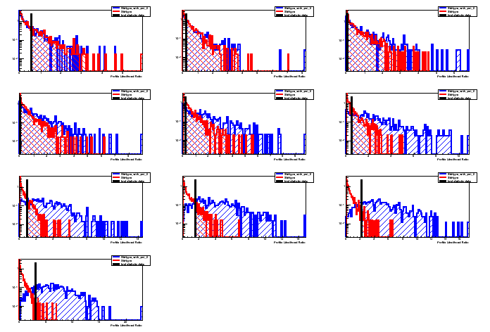
Starting from the null hypothesis no third peak is present, start by
dialing in some signal in small steps and for each step generate
pesudo data and fit it according to both the null and the
alternative hypothesis and perform a p value scan. Then calculate
the ratio of the p-values and whenever the ratio crosses the 0.05
line you can read the 95% CONFIDENCE LEVEL upper limit.
I will show results for both the asymptotic calculation using the Asymov dataset (somewhat fast) and also the famous CLs criterium. There’s a third method called the Feldman-Cousins that I will explain later.
Asymtotic 68 %

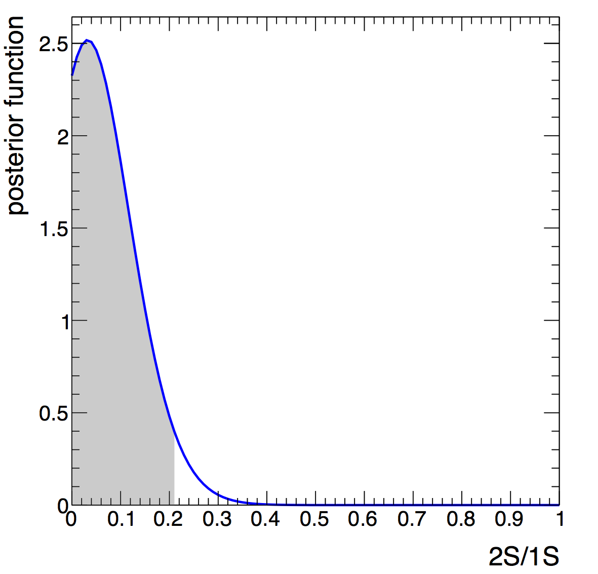
Bayesian approach:
Just assume a probabilty distribution for the parameter of interest
and use Bayesian theorem to posterior probability. Find the value
you need to integrate to in order to make the posterior 0.95. Or in
other words, 95% CREDIBLE INTERVAL upper limit.
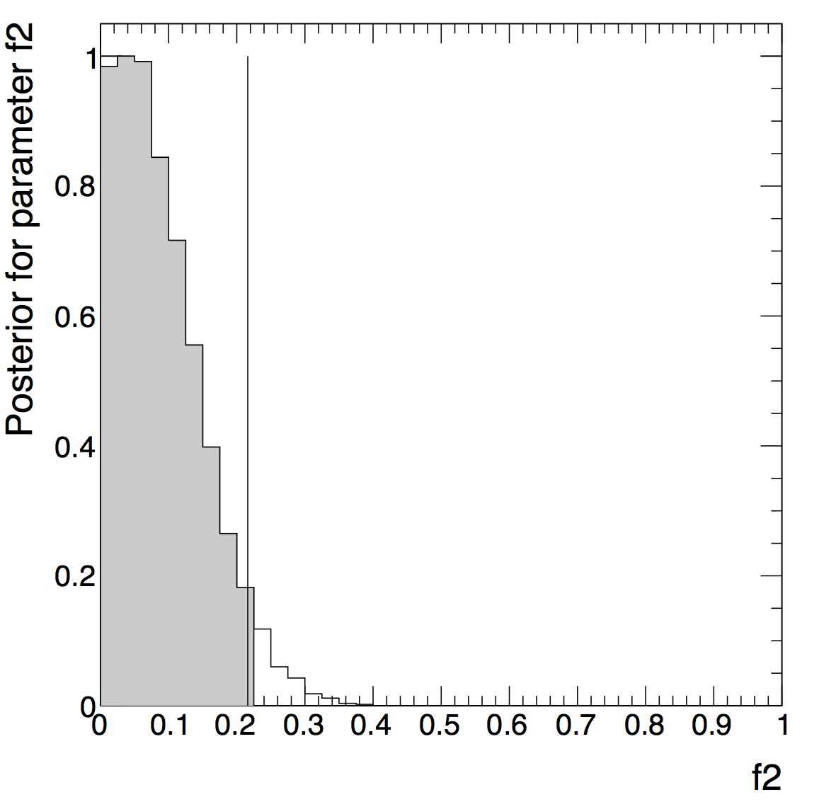
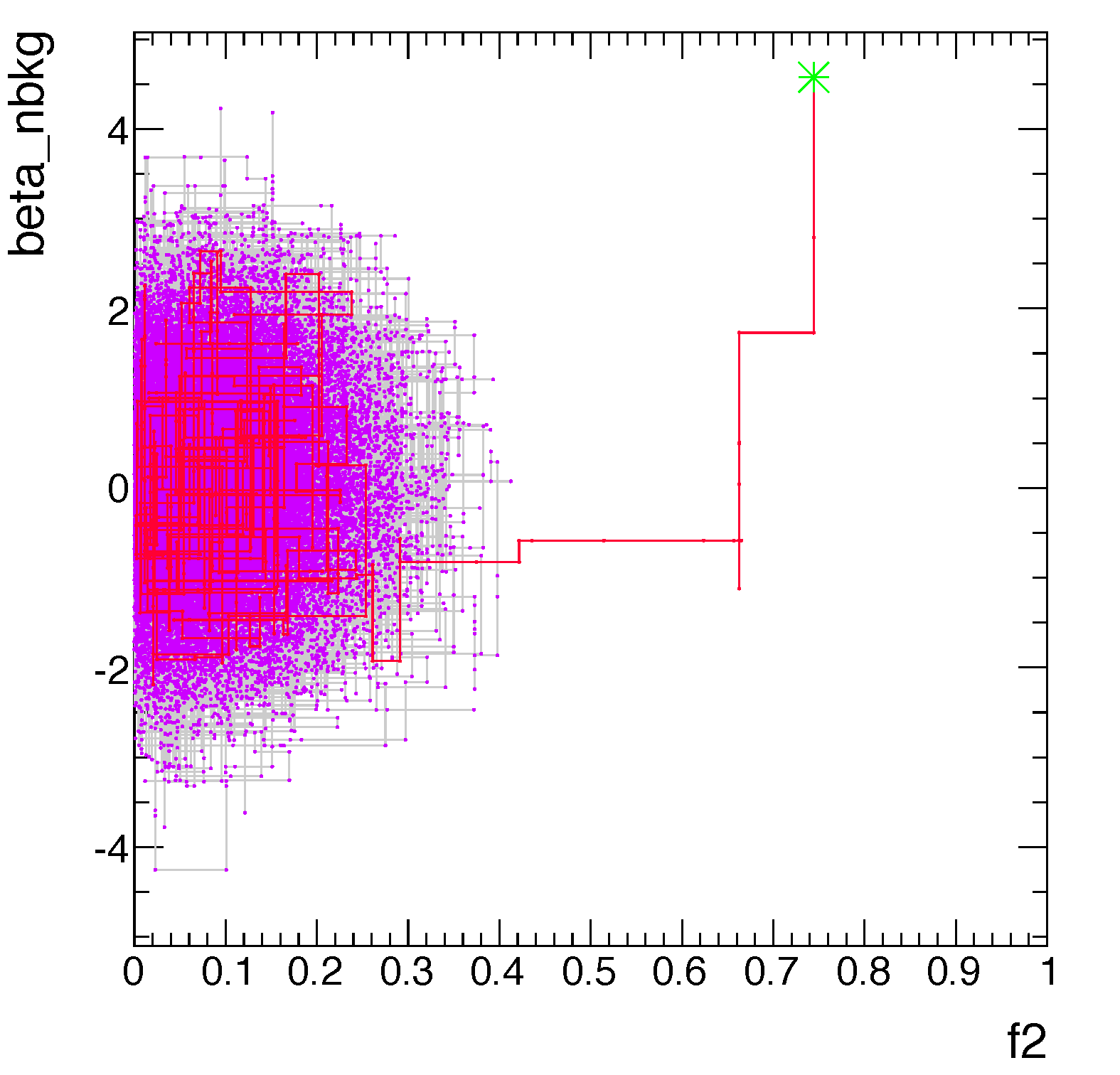
For the Bayesian we will use both the numerical posterior and the Markov Chain Montecarlo.
For the numerical posterior
For the Markov Chain Montecarlo.
Let’s do this in ROOT and let’s take advantage of ROOFIT and ROOSTATS.
Start with your header files:
#ifndef __CINT__
#include "RooGlobalFunc.h"
#endif
#include "RooDataSet.h"
#include "RooRealVar.h"
#include "RooGaussian.h"
#include "RooAddPdf.h"
#include "RooProdPdf.h"
#include "RooAddition.h"
#include "RooProduct.h"
#include "TCanvas.h"
#include "RooChebychev.h"
#include "RooAbsPdf.h"
#include "RooFit.h"
#include "RooFitResult.h"
#include "RooPlot.h"
#include "RooAbsArg.h"
#include "RooWorkspace.h"
#include "RooStats/ProfileLikelihoodCalculator.h"
#include "RooStats/HypoTestResult.h"
#include <string>
Now we use this for safety on library loading:
using namespace RooFit;
using namespace RooStats;
See below for implementation:
void AddModel(RooWorkspace*);
void AddData(RooWorkspace*);
void DoHypothesisTest(RooWorkspace*);
void MakePlots(RooWorkspace*);
The main macro:
 void three_peaks() {

 // Create a workspace to manage the project.
 RooWorkspace* wspace = new RooWorkspace("wks");

 // add the signal and background models to the workspace
 AddModel(wspace);

 // add some toy data to the workspace
 AddData(wspace);

 // inspect the workspace if you wish
 //  wspace->Print();

 // do the hypothesis test
 DoHypothesisTest(wspace);

 // make some plots
 MakePlots(wspace);

 // cleanup
 delete wspace;
}
Now let’s add our model. As stated above: polynomial background and three Crystal Ball functions for the the signal:
void AddModel(RooWorkspace* wks){

double const M1S(9.460);
double const M2S(10.023);
double const M3S(10.355);

// set range of observable
Double_t lowRange = 7, highRange = 14;

// make a RooRealVar for the observable
RooRealVar invMass("invMass", "M_{inv}", lowRange, highRange,"GeV");

/////////////////////////////////////////////
// make Upsilon1S model.  Just like signal model
RooRealVar m1S("m1S", "Upsilon1S Mass", M1S, 7, 14);
RooRealVar sigma1("sigma1","Width of Gaussian",0.08,0.,1.2)  ;
RooGaussian nsig1S("nsig1S", "nsig1S Model", invMass, m1S, sigma1);
// we know Upsilon1S mass
m1S.setConstant();
// assume we know resolution too
sigma1.setConstant();


/////////////////////////////////////////////
// make a simple signal model.
RooRealVar m2S("m2S","Upsilon Mass",M2S,7,14) ;
RooRealVar sigma2("sigma2","Width of Gaussian",0.08,0.,1.2)  ;
RooGaussian nsig2S("nsig2S", "Signal Model", invMass, m2S, sigma2);
// we will test this specific mass point for the signal
m2S.setConstant();
// and we assume we know the mass resolution
sigma2.setConstant();

// make a simple signal model.
RooRealVar m3S("m3S","Upsilon Mass", M3S, 7,14) ;
RooRealVar sigma3("sigma3","Width of Gaussian", 0.08, 0.,1.2)  ;
RooGaussian nsig3S("nsig3S", "Signal Model", invMass, m3S, sigma3);
// we will test this specific mass point for the signal
m3S.setConstant();
// and we assume we know the mass resolution
sigma3.setConstant();


//////////////////////////////////////////////
// make background model
RooRealVar a0("a0","a0",0.26,-1,1) ;
RooRealVar a1("a1","a1",-0.17596,-1,1) ;
RooRealVar a2("a2","a2",0.018437,-1,1) ;
RooRealVar a3("a3","a3",0.02,-1,1) ;
RooChebychev likeSignModel("likeSignModel","Polynomail background",invMass,RooArgList(a0,a1,a2)) ;

// let's assume this shape is known, but the normalization is not
a0.setConstant();
a1.setConstant();
a2.setConstant();

//////////////////////////////////////////////
// combined model

// Setting the fraction of Upsilon1S to be 40% for initial guess.
RooRealVar f1S("f1S","fraction of 1S background events", 0.3, 0., 1) ;

// Setting the fraction of Upsilon1S to be 8% for initial guess.
RooRealVar f2S("f2S","fraction of 2S background events", 0.07, 0., 1) ;

RooRealVar x3("x3", "#chi_{2}", 0.01, 0. ,1.);

// Set the Upsilon3S fraction of signal to 2.5%.
//RooRealVar fsigExpected("fsigExpected","expected fraction of signal events",0.025,0.,1) ;
RooFormulaVar fsigExpected("fsigExpected", "@0*@1", RooArgList(x3, f1S));

//RooRealVar fsigExpected("fsigExpected","expected fraction of signal events",0.01,0.,1) ;
//fsigExpected.setConstant(kTRUE); // use mu as main parameter, so fix this.

//RooFormulaVar f3_hi("f3_hi","@0/@1",RooArgList(nsig2S,nsig1S));


// Introduce mu: the signal strength in units of the expectation.
// eg. mu = 1 is there's a signal, mu = 0 is no signal, mu=2 is 2x the SM
RooRealVar mu("mu","signal strength in units of SM expectation",1,0.,2) ;
mu.setConstant(kFALSE);

// Introduce ratio of signal efficiency to nominal signal efficiency.
// This is useful if you want to do limits on cross section.
RooRealVar ratioSigEff("ratioSigEff","ratio of signal efficiency to nominal signal efficiency",1. ,0.,2) ;
ratioSigEff.setConstant(kTRUE);

// finally the signal fraction is the product of the terms above.

RooProduct fsig("fsig","fraction of signal events",RooArgSet(mu,ratioSigEff,fsigExpected)) ;

wks->factory( "nbkg_nom[0.1]" );
wks->factory( "nbkg_kappa[1.10]" );
wks->factory( "cexpr::alpha_nbkg('pow(nbkg_kappa,beta_nbkg)',nbkg_kappa,beta_nbkg[0,-5,5])" );
wks->factory( "prod::nbkg(nbkg_nom,alpha_nbkg)" );
wks->factory( "Gaussian::constr_nbkg(beta_nbkg,glob_nbkg[0,-5,5],1)" );

RooAbsPdf* LSBackground = wks->pdf("constr_nbkg");
// full model
RooAddPdf model("model","model 1S+2S+3S +bgd",RooArgList(nsig3S,nsig2S,nsig1S,*LSBackground ),RooArgList(fsig,f2S,f1S)) ;
RooAddPdf model_bg("model_bg","model 1S+2S+bgd",RooArgList(nsig2S,nsig1S,*LSBackground ),RooArgList(fsig,f2S,f1S)) ;


// interesting for debugging and visualizing the model
model.printCompactTree("","fullModel.txt");
model.graphVizTree("fullModel.dot");

wks->import(model);
}