Analysis

Fitting R(t), the MC ratio

**Table 1:** Fitting Summary Summary of the &chi²/dof for fits as presented above and extracted c parameters (where c =1 corresponds to expected degree of interference and c=0 corresponds to no interference). The statistical error associated with the c parameter is multiplied by a correction factor defined as the SQRT of the &chi²/dof. In addition the difference between the statistical error and the 'corrected' error is taken in the last column.
Dataset/Fit	Rapidity	&chi²/dof	c	statistical error × correction	Excess Error
Minbias/par5	0 < y < 0.5	44.2/47	0.9539±0.076	0.074	-0.002
Minbias/par5	0.5 < y < 1.0	80.18/47	0.9275±0.110	0.144	0.034
Minbias/par6	0 < y < 0.5	46.11/47	0.9485±0.076	0.075	-0.001
Minbias/par6	0.5 < y < 1.0	80.04/47	0.9224±0.109	0.142	0.033
Minbias/pol5	0 < y < 0.5	45.88/47	0.9507±0.076	0.075	-0.001
Minbias/pol5	0.5 < y < 1.0	81.67/47	0.9266±0.110	0.145	0.074
Minbias/pol6	0 < y < 0.5	46.28/47	0.9479±0.076	0.075	-0.001
Minbias/pol6	0.5 < y < 1.0	79.16/47	0.9287±0.110	0.143	0.033
Topology/par5	0.1 < y < 0.5	87.73/47	0.8223±0.120	0.164	0.044
Topology/par5	0.5 < y < 1.0	85.09/47	1.048±0.209	0.281	0.072
Topology/par6	0.1 < y < 0.5	80.58/47	0.8381±0.114	0.153	0.039
Topology/par6	0.5 < y < 1.0	85.21/47	0.9966±0.199	0.261	0.062
Topology/pol5	0.1 < y < 0.5	90.63/47	0.8212±0.124	0.172	0.048
Topology/pol5	0.5 < y < 1.0	84.53/47	1.081±0.213	0.286	0.073
Topology/pol6	0.1 < y < 0.5	83.05/47	0.8371±0.119	0.158	0.039
Topology/pol6	0.5 < y < 1.0	87.9/47	0.9637±0.2039	0.279	0.075

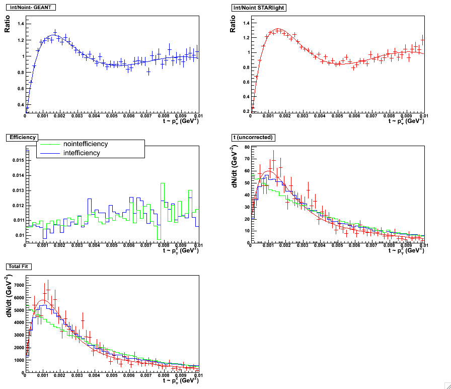
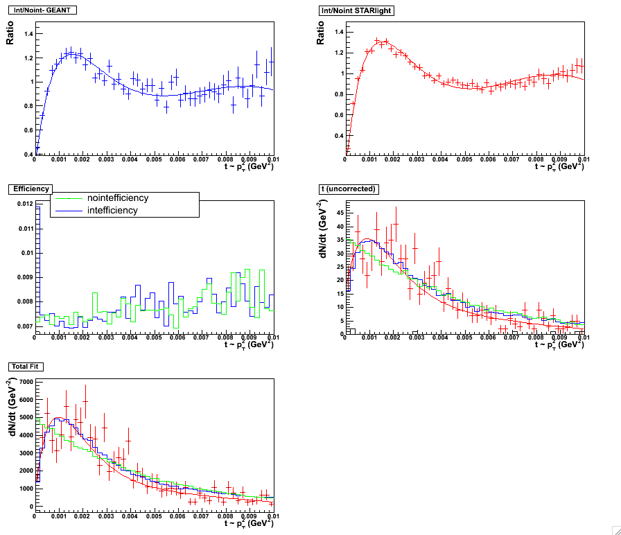
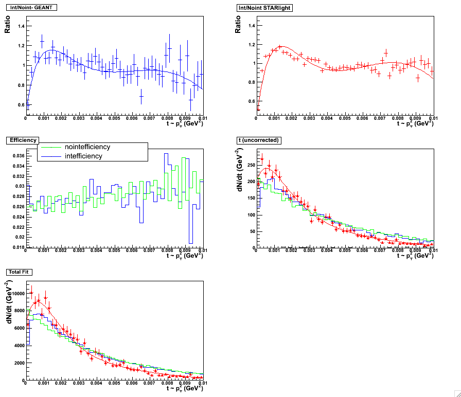
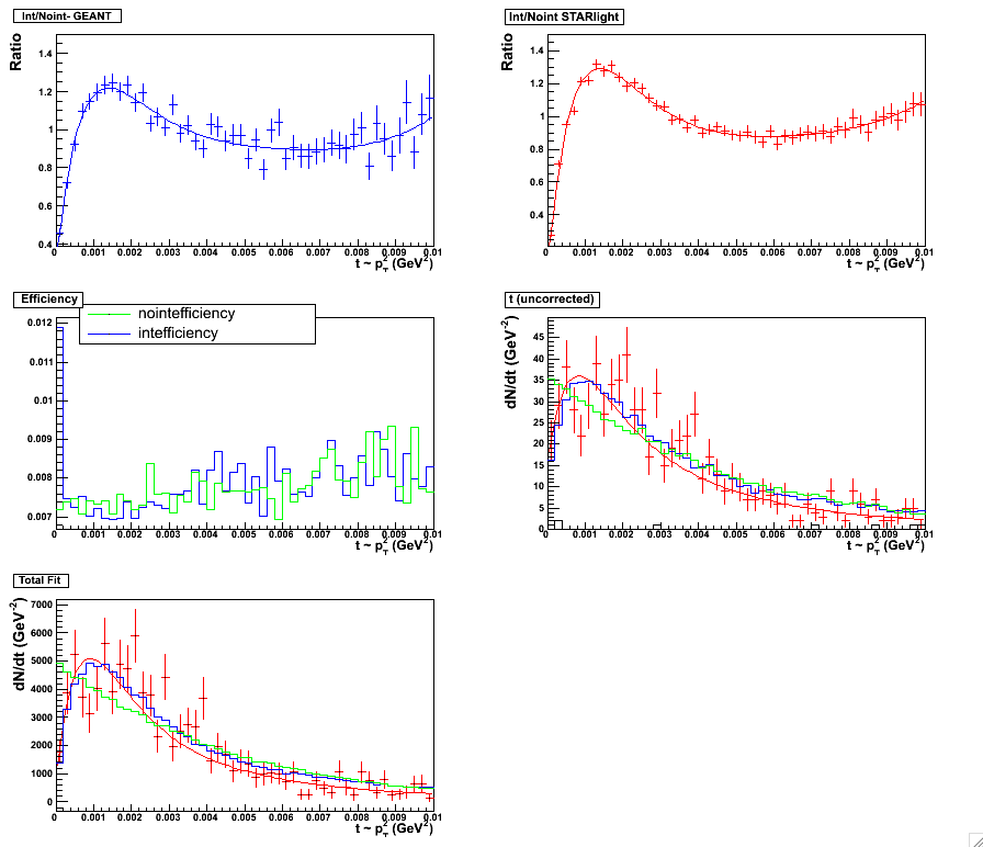
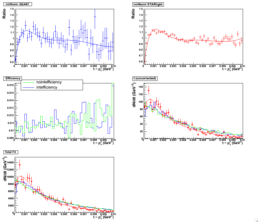
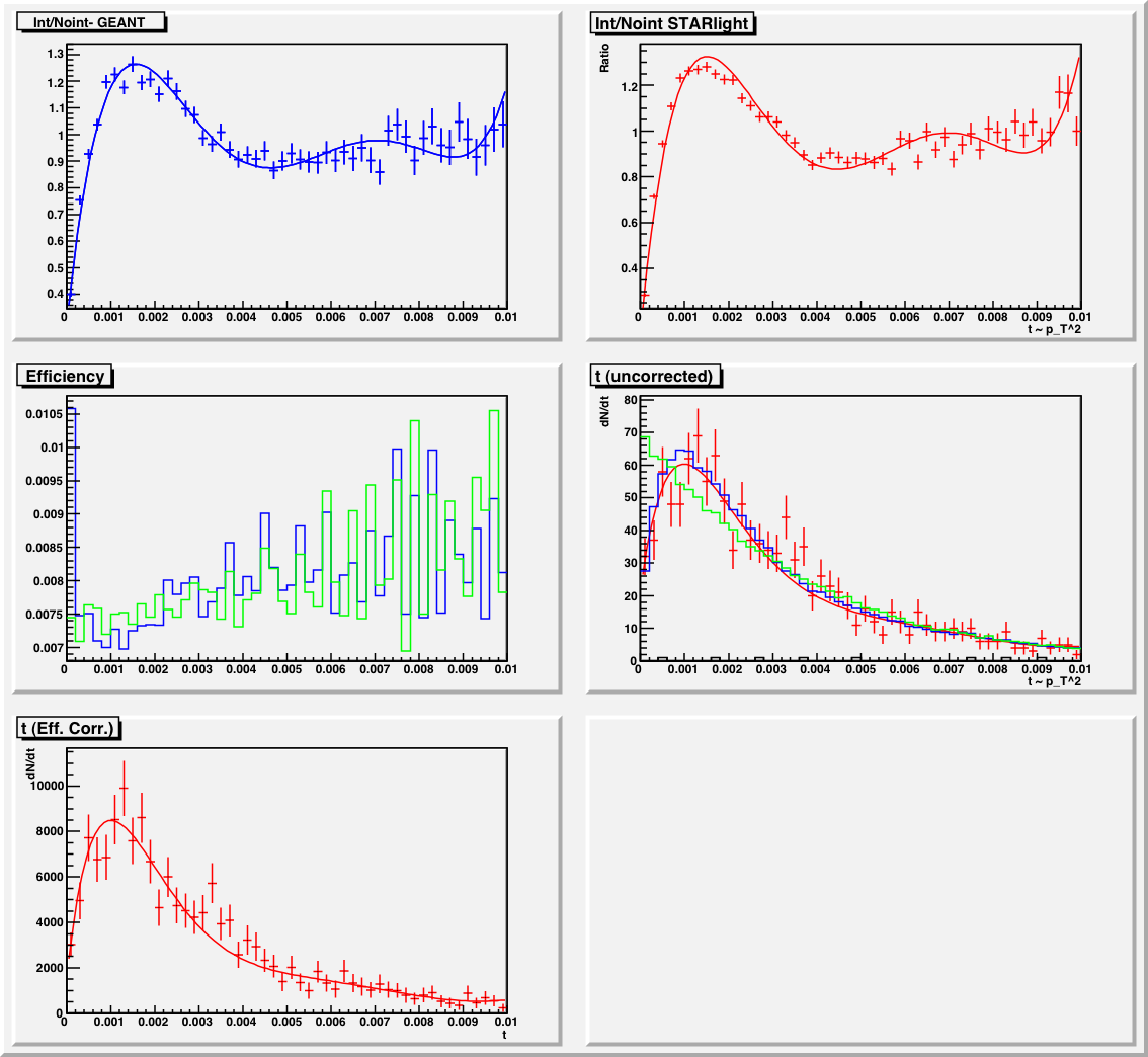
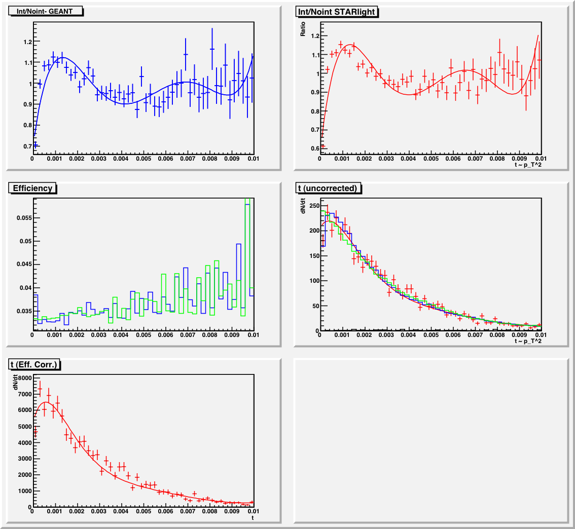
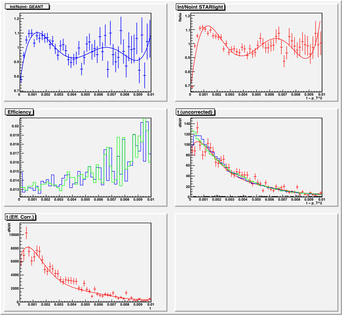
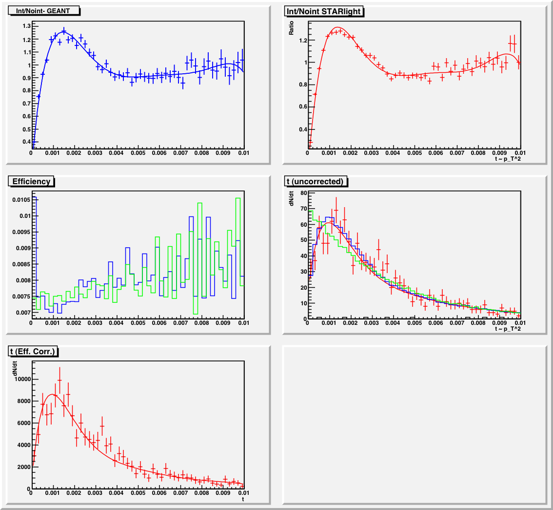
A. 5 Parameter Fits

Figure 1:

Fitting scheme for the minbias set, 0.1 < y < 0.5. Plot with statistics here.

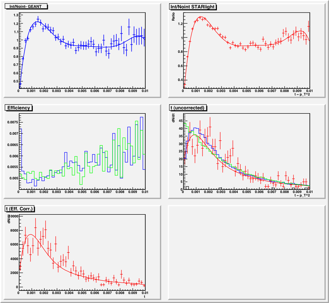
Figure 2:

Fitting scheme for the minbias set, 0.5 < y < 1.0. Plot with statistics here.

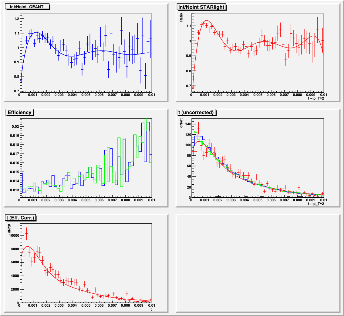
Figure 3:

Fitting scheme for the topology set, 0.1 < y < 0.5. Plot with statistics here.

Figure 4:

Fitting scheme for the topology set, 0.5 < y < 1.0. Plot with statistics here.

B. 6 Parameter Fits

Figure 5:

Fitting scheme for the minbias set, 0.1 < y < 0.5. Plot with statistics here.

Figure 6:

Fitting scheme for the minbias set, 0.5 < y < 1.0. Plot with statistics here.

Figure 7:

Fitting scheme for the topology set, 0.1 < y < 0.5. Plot with statistics here.

Figure 8:

Fitting scheme for the topology set, 0.5 < y < 1.0. Plot with statistics here.

C. 5th Order Polynomial Fits

Figure 9:

Fitting scheme for the minbias set, 0.1 < y < 0.5. Plot with statistics here.

Figure 10:

Fitting scheme for the minbias set, 0.5 < y < 1.0. Plot with statistics here.

Figure 11:

Fitting scheme for the topology set, 0.1 < y < 0.5. Plot with statistics here.

Figure 12:

Fitting scheme for the topology set, 0.5 < y < 1.0. Plot with statistics here.

C. 6th Order Polynomial Fits

Figure 13:

Fitting scheme for the minbias set, 0.1 < y < 0.5. Plot with statistics here.

Figure 14:

Fitting scheme for the minbias set, 0.5 < y < 1.0. Plot with statistics here.

Figure 15:

Fitting scheme for the topology set, 0.1 < y < 0.5. Plot with statistics here.

Figure 16:

Fitting scheme for the topology set, 0.5 < y < 1.0. Plot with statistics here.