Fitting
Fitting R(t), the MC ratio
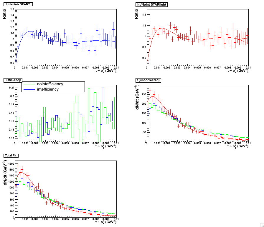
We model the interference
with events generated with our Monte Carlo generator, STARlight. Two sets are
generated, one with interference and one without. A ratio is arrived at by dividing
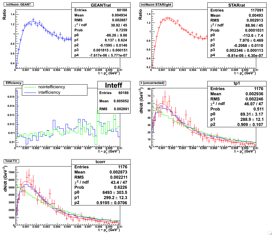
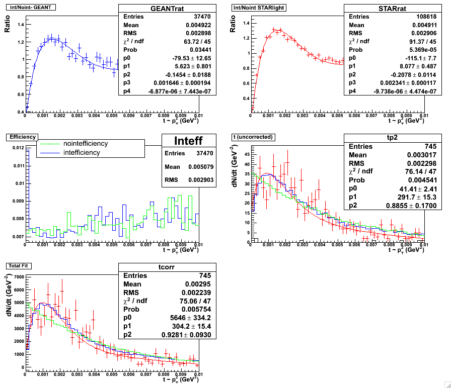
the t spectra of the sets. The ratio is then fit with a function [R(t)]
which figures into the overall fit applied to the data:
Ae-kt(1+c[R(t)-1]). Various fitting functions, (five parameter fit,
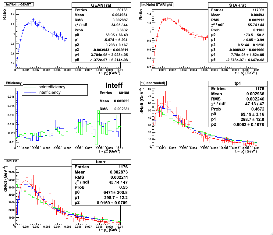
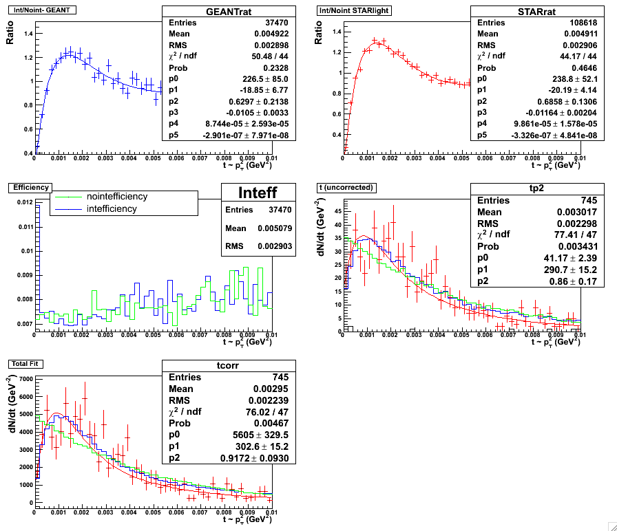
six parameter fit,
fifth order polynomial, and sixth order polynomial fit) have been tried in order to
optimize the fit and assess systematic error.
Table 1:
Fitting Summary Summary of the &chi2/dof for
fits as presented below and extracted c parameters (where c =1 corresponds to expected degree of interference
and c=0 corresponds to no interference). When the &chi2/dof is significantly greater than 1,
the statistical error associated with the c parameter is multiplied by
a correction factor defined as the SQRT of the &chi2/dof as per a method prescribed in the particle
data book. In addition the difference between
the statistical error and the 'corrected' error is taken in the last column.
| Dataset/Fit | Rapidity | &chi²/dof | c | statistical error × correction | Excess Error |
| Minbias/par5 |
0 < y < 0.5 | 44.2/47 | 0.9539±0.076 | n/a | -0.002 |
|---|
| 0.5 < y < 1.0 | 80.18/47 | 0.9275±0.110 | 0.144 | 0.034 |
| Minbias/par6 |
0 < y < 0.5 | 46.11/47 | 0.9485±0.076 | n/a | -0.001 |
|---|
| 0.5 < y < 1.0 | 80.04/47 | 0.9224±0.109 | 0.142 | 0.033 |
| Minbias/pol5 |
0 < y < 0.5 | 45.88/47 | 0.9507±0.076 | n/a | -0.001 |
|---|
| 0.5 < y < 1.0 | 81.67/47 | 0.9266±0.110 | 0.145 | 0.074 |
| Minbias/pol6 |
0 < y < 0.5 | 46.28/47 | 0.9479±0.076 | n/a | -0.001 |
|---|
| 0.5 < y < 1.0 | 79.16/47 | 0.9287±0.110 | 0.143 | 0.033 |
| Topology/par5 |
0.1 < y < 0.5 | 87.73/47 | 0.8223±0.120 | 0.164 | 0.044 |
|---|
| 0.5 < y < 1.0 | 85.09/47 | 1.048±0.209 | 0.281 | 0.072 |
| Topology/par6 |
0.1 < y < 0.5 | 80.58/47 | 0.8381±0.114 | 0.153 | 0.039 |
|---|
| 0.5 < y < 1.0 | 85.21/47 | 0.9966±0.199 | 0.261 | 0.062 |
| Topology/pol5 |
0.1 < y < 0.5 | 90.63/47 | 0.8212±0.124 | 0.172 | 0.048 |
|---|
| 0.5 < y < 1.0 | 84.53/47 | 1.081±0.213 | 0.286 | 0.073 |
| Topology/pol6 |
0.1 < y < 0.5 | 83.05/47 | 0.8371±0.119 | 0.158 | 0.039 |
|---|
| 0.5 < y < 1.0 | 87.9/47 | 0.9637±0.2039 | 0.279 | 0.075 |
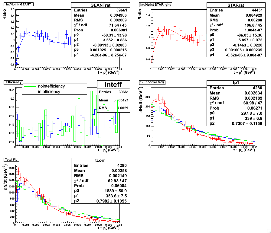
A. Minbias Fits
Figure 1 & 2:
Five Parameter fit. Fitting scheme for the minbias set, 0.0 < y < 0.5. Plot with statistics
here. (left panel)
Five Parameter fit. Fitting scheme for the minbias set, 0.5 < y < 1.0. Plot with statistics
here. (right panel)
 |
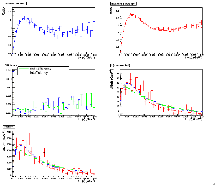 |
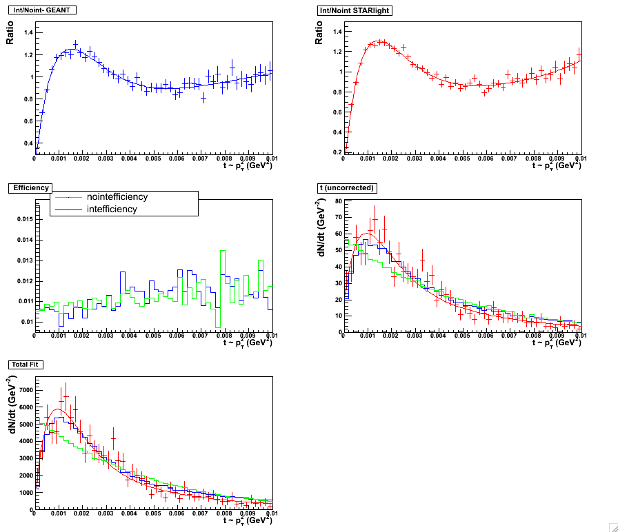
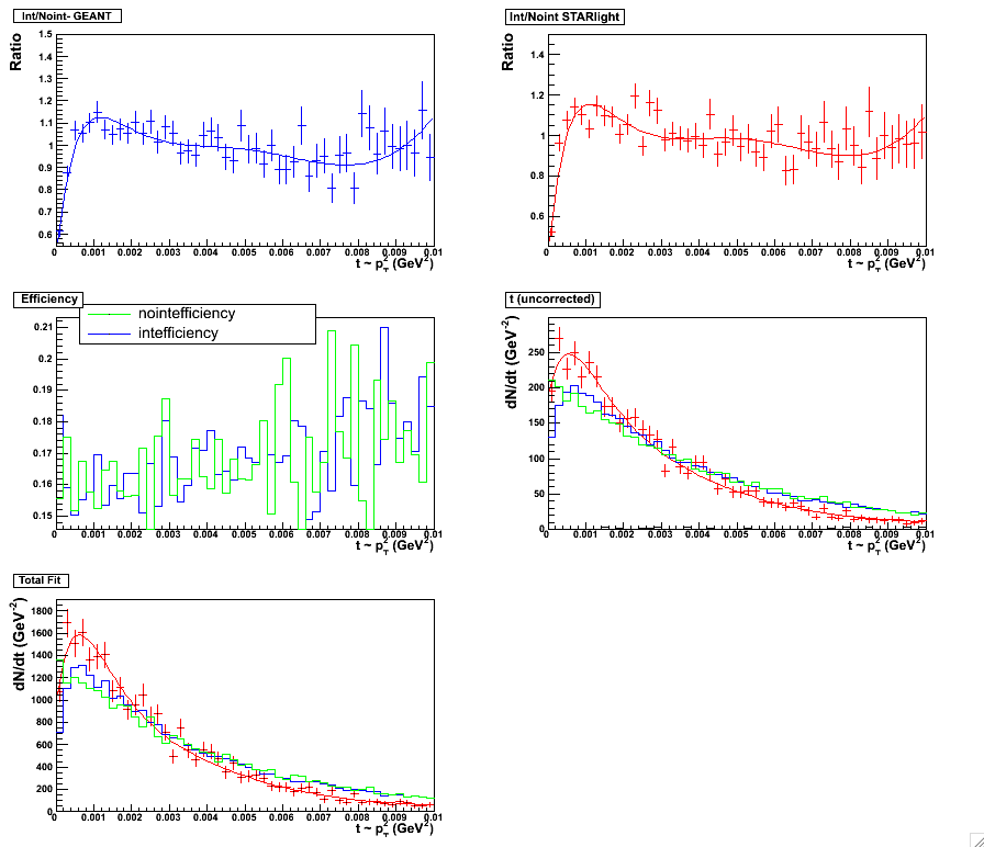
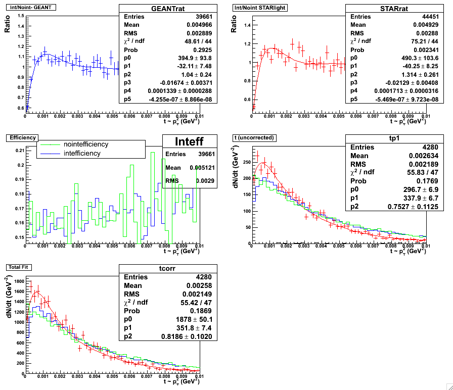
Figure 3 & 4:
Six Parameter fit. Fitting scheme for the minbias set, 0.0 < y < 0.5. Plot with statistics
here. (left panel)
Six Parameter fit. Fitting scheme for the minbias set, 0.5 < y < 1.0. Plot with statistics
here. (right panel)
 |
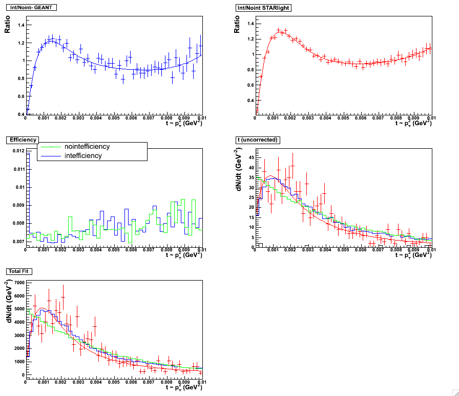 |
Figure 5 & 6:
Fifth order polynomial fit. Fitting scheme for the minbias set, 0.0 < y < 0.5. Plot with statistics
here. (left panel)
Fifth order polynomial fit. Fitting scheme for the minbias set, 0.5 < y < 1.0. Plot with statistics
here. (right panel)
 |
 |
Figure 7 & 8:
Sixth order polynomial fit. Fitting scheme for the minbias set, 0.0 < y < 0.5. Plot with statistics
here. (left panel)
Sixth order polynomial fit. Fitting scheme for the minbias set, 0.5 < y < 1.0. Plot with statistics
here. (right panel)
 |
 |
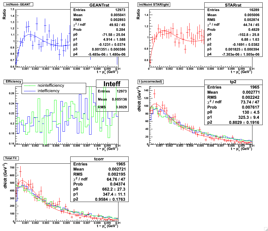
B. Topology Fits
Figure 9 & 10:
Five Parameter fit. Fitting scheme for the topology set, 0.05 < y < 0.5. Plot with statistics
here. (left panel)
Five Parameter fit. Fitting scheme for the topology set, 0.5 < y < 1.0. Plot with statistics
here. (right panel)
 |
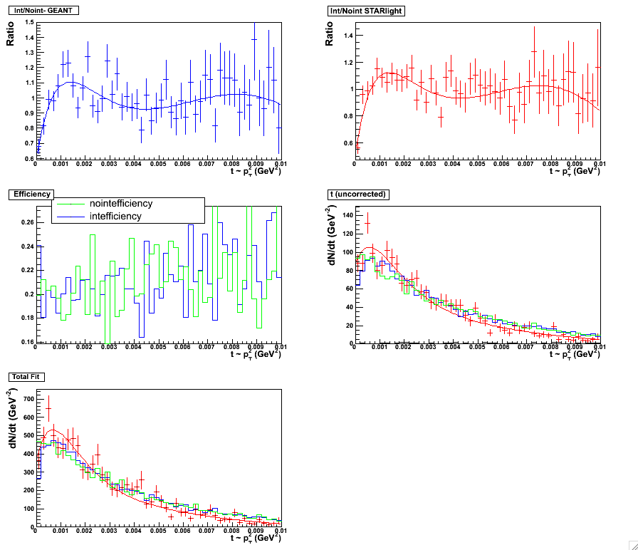 |
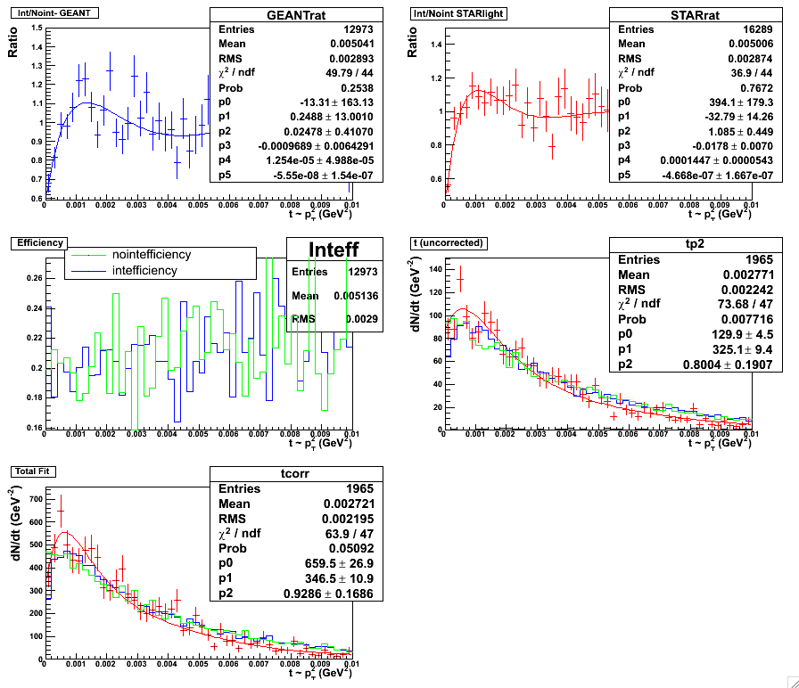
Figure 11 & 12:
Six Parameter fit. Fitting scheme for the topology set, 0.05 < y < 0.5. Plot with statistics
here. (left panel)
Six Parameter fit. Fitting scheme for the topology set, 0.5 < y < 1.0. Plot with statistics
here. (right panel)
 |
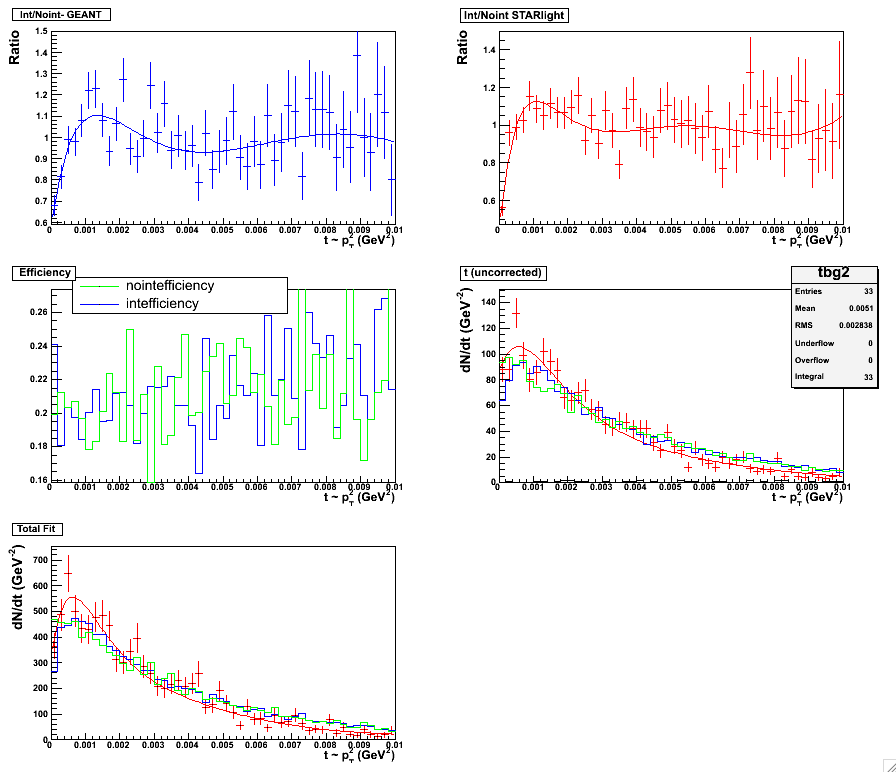 |
Figure 13 & 14:
Fifth order polynomial fit. Fitting scheme for the topology set, 0.05 < y < 0.5. Plot with statistics
here. (left panel)
Fifth order polynomial fit. Fitting scheme for the topology set, 0.5 < y < 1.0. Plot with statistics
here. (right panel)
 |
 |
Figure 14 & 15:
Sixth order polynomial fit. Fitting scheme for the topology set, 0.05 < y < 0.5. Plot with statistics
here. (left panel)
Sixth order polynomial fit. Fitting scheme for the topology set, 0.5 < y < 1.0. Plot with statistics
here. (right panel)
 |
 |