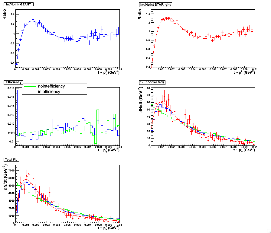
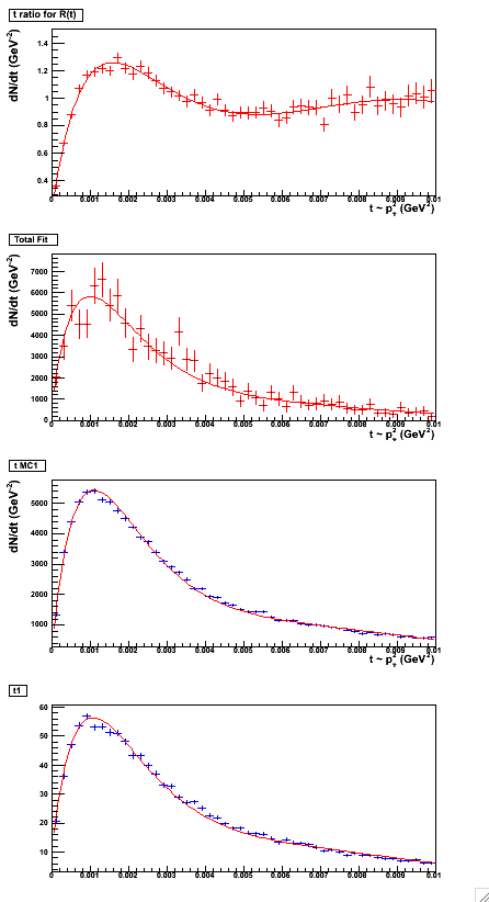
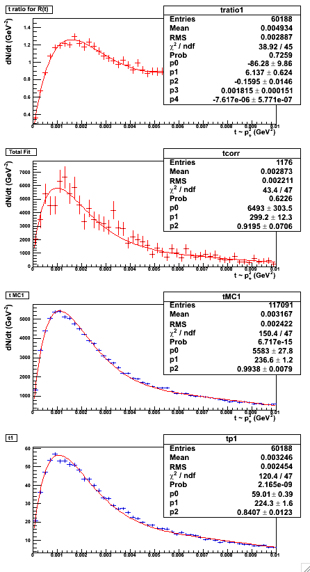
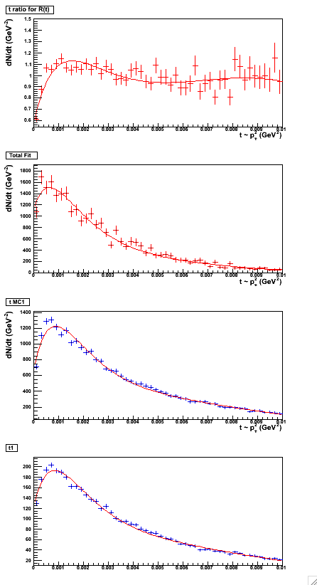
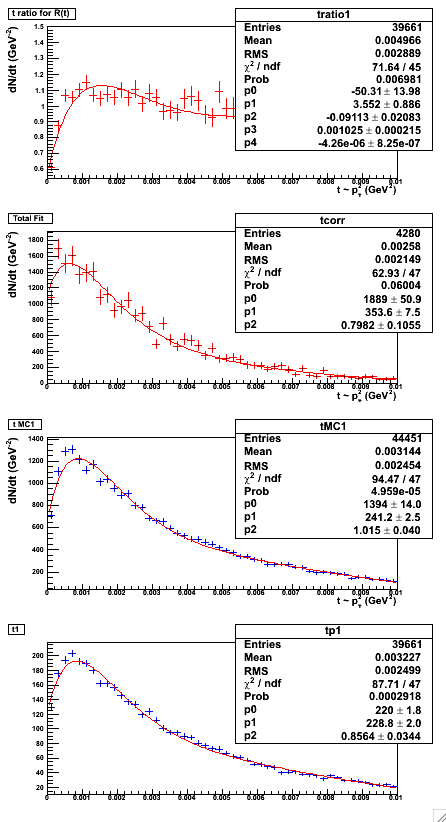
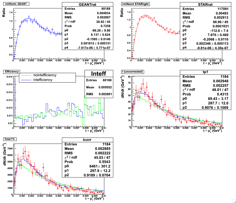
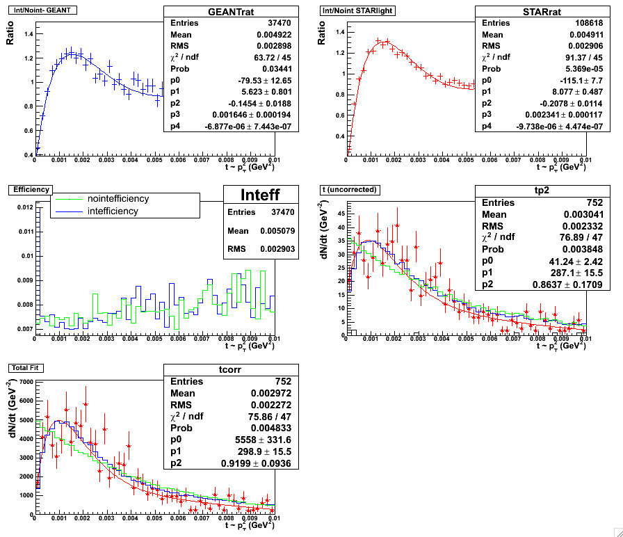
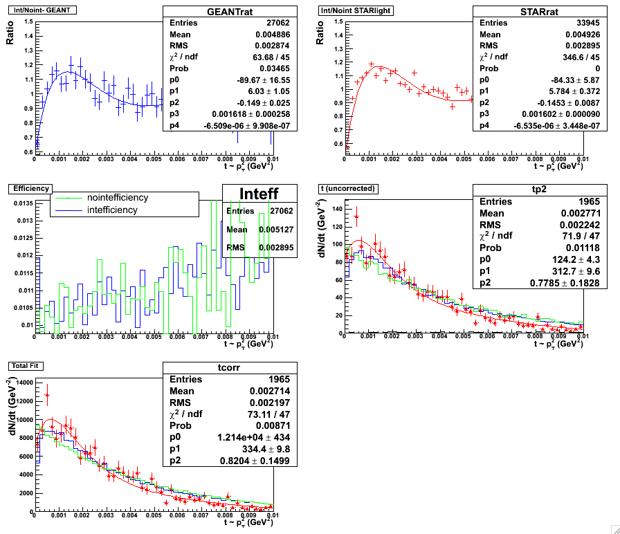
Five Parameter fit. Fitting scheme for the minbias set, 0.0 < y < 0.5. Plot with statistics here. (left panel)
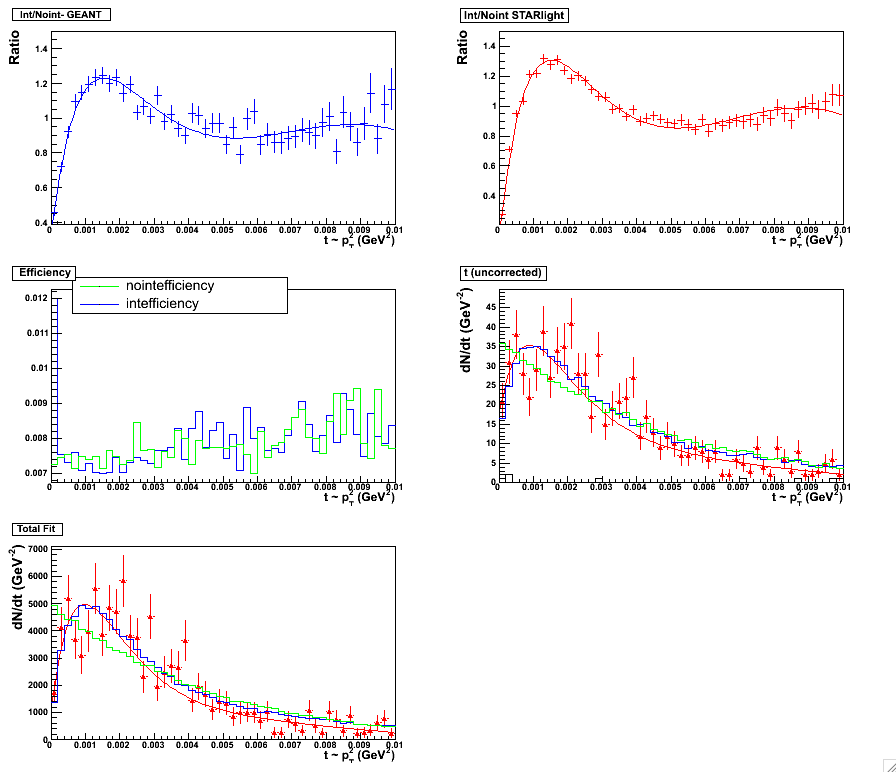
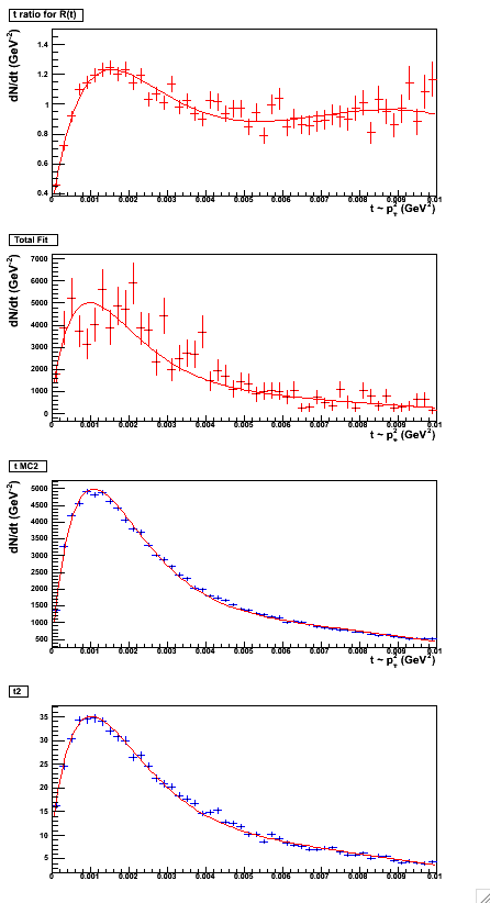
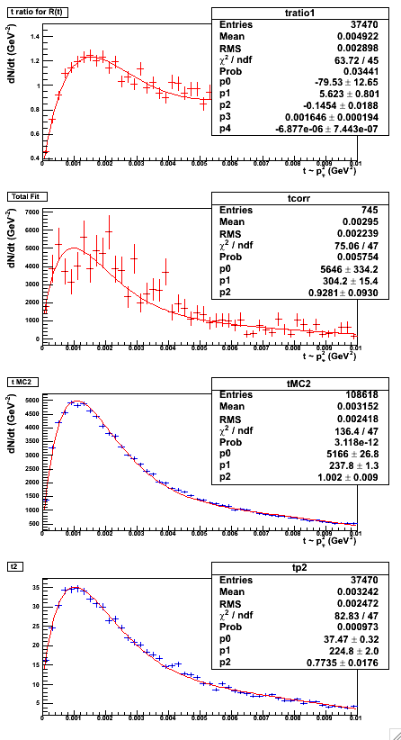
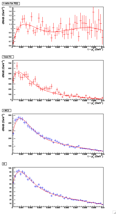
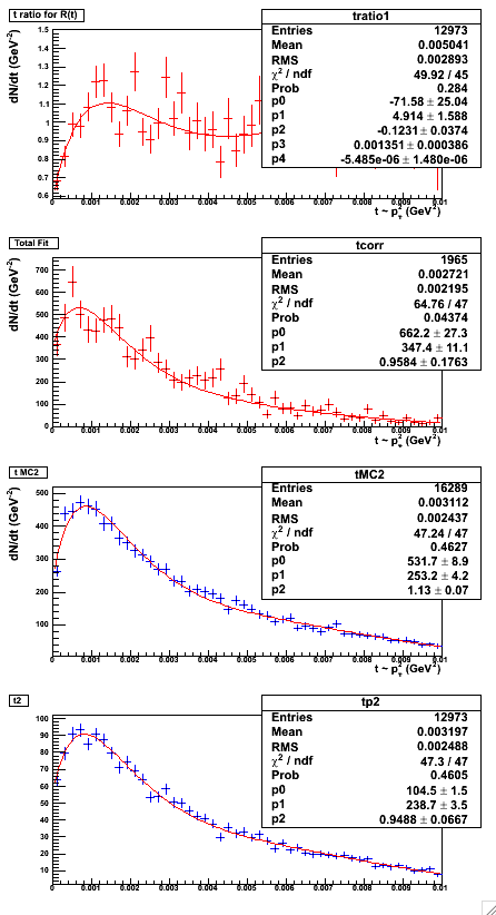
Five Parameter fit. Fitting scheme for the minbias set, 0.5 < y < 1.0. Plot with statistics here. (right panel)
| Source of Error | Estimated Value |
| Forward/Back Comparison | |
| Cosmics | 0% |
| Ratio Fits | |
| Slope Fits | 1% |
| Theory |
We rerun the analysis with the requirement that pairs be unlike-sign removed and note how much doubling the background affects the results.
|
|
 |
 |
 |
 |
 |
 |
 |
 |
 |
 |
| Fit | Error |
| minbias 0 < y < 0.5 | 0.00271 |
| minbias 0.5 < y < 1.0 | 0.00327 |
| topology 0.1 < y < 0.5 | 0.00917 |
| topology 0.5 < y < 1.0 | 0.0523 |
| Dataset | 100% | 90% | 80% |
| minbias 0 < y < 0.5 | 1.01 | 1.00 | 0.99 |
| minbias 0.5 < y < 1.0 | 0.92 | 0.91 | 0.91 |
| topology 0.1 < y < 0.5 | 0.83 | 0.83 | 0.87 |
| topology 0.5 < y < 1.0 | 1.04 | 1.04 | 1.10 |
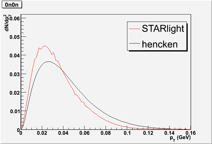
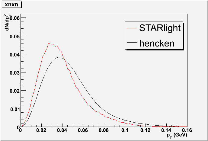
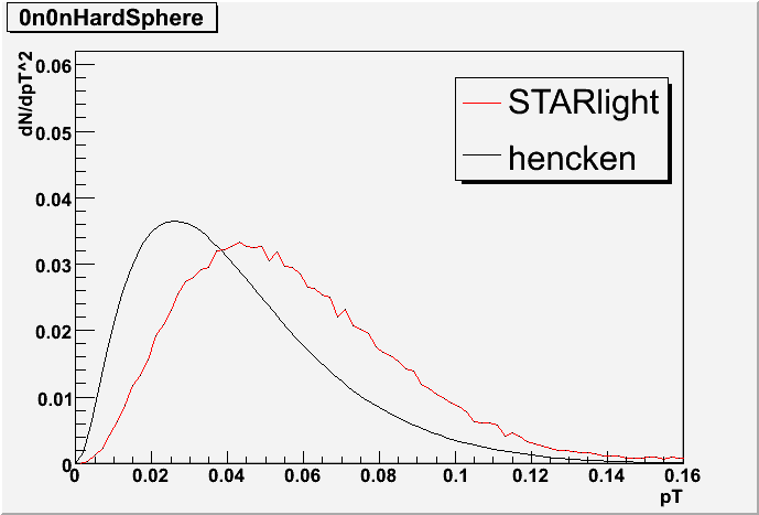
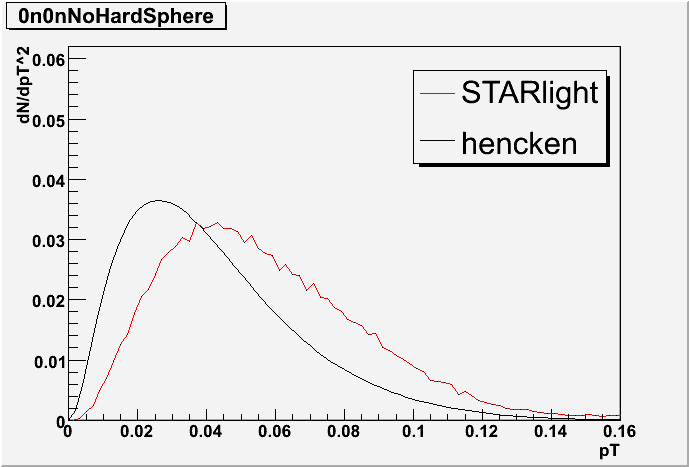
Two main models predict and describe the interference effect we see in the data. STARlight is the Monte Carlo event generator algorithm which is used in this analysis. It is based on theory and calculations by Klein and Nystrand. The other model is by Hencken, Baur, and Trautmann (HBT) .
KNLite Comparisons
Extensive predictions and comparisons have been made with the KNLite model by Jim Draper.STARlight Comparisons
Figure 1 & 2:
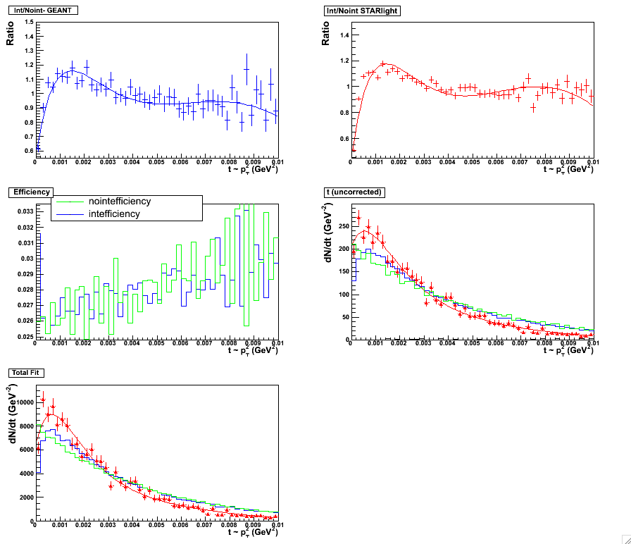
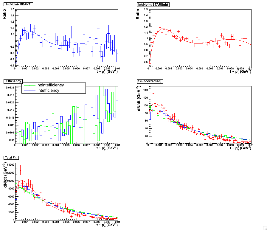
Figure 3 & 4: